The Cocktail Party Effect (Part 1 of 2)

Late at night, when the boys are (finally) asleep, we sometimes like to watch stuff on the television.  If the TV is too loud, the boys wake up, and that really breaks immersion.  If the TV is too quiet, we can't hear the gripping dialogue, and that breaks immersion too.

  Here's how I fixed it in code.

Mono

Okay. Don't judge me, but the first thing I did is to convert the incoming stereo audio down to mono.  Most music tends to be well spatialised, while the voice track comes through the center channel.  By converting to mono I estimate a ~3dB drop in perceived volume during musical interludes, or, conversely, I can raise the total volume by 3dB without waking up the boys.

Bass

The next thing to do is to cut the low frequencies.  The rumbles and the explosions.  The ones which reverberate throughout the house and wake up the kids and the neighbors too.

It's relatively easy to find info on constructing a digital high-pass filter on the internet, provided you can cut through the jargon.  Generally there tends to be an incoming signal, denoted as x_n.  It's the series of samples coming from your video decoder.  And then there's an outgoing signal, y_n.  It's the series of samples that you send to the sound card.

Then there's some function that links them together.  Here's an example of a really simple high-pass filter you can find on the internet :

y_n = 0.2 . x_n  + 0.8 . y_n-1

It's a simple matter to turn this into code:

A simple high-pass filter, in C++.

Z-transform

To work out the frequency response, we can use the Z-transform to find the Transfer Function, which maps our filter from the discrete, time domain, into the continuous, frequency domain.  In our case:

H(z) = Y(z)/X(z) =  0.2 / (1 + 0.8 . z^-1)

The cool thing is we can use theory to treat z like a complex number, even though in practice, all the x_n and y_n will be floating point numbers.  For example, to compute the frequency response at 1000Hz, with a sample rate of 48kHz, we take:

i = √-1

FrequencyResponse(1000Hz) = | H(2π1000/48000 i) |

= | 0.2/(1 + 0.8 / (2π1000i/48000) ) |

= 0.008

If we draw this on a graph, with frequency (Hz) on the X-axis, and magnitude (dB) on the Y-axis, we can get a "Bode Plot" of our filter:

A Bode Plot for a simple filter.

So that's a great start, but now we want more control over which frequencies pass through the filter, and which are blocked, and by how much.

Optimize

Back in the old days, we would have had to endlessly try different filter combinations and painstakingly compute Bode plots to find combinations of filters that might fit our requirements.

But now that we all have super-computers under our desks, we've got much more powerful tools to solve an old problem in a new way.

In pseudo-code, it looks like this :

def GetDesiredFrequencyResponse(frequency):

    // Your desired EQ function goes here

def EvaluateFilter(filter):

    errorSum = 0

    for frequency in 20 .. 22000:

        freq1 = GetDesiredFrequencyResponse(frequency)

        freq2 = filter.CalcFrequencyResponse(frequency)

        errorTerm = freq1 - freq2

        errorSum += errorTerm * errorTerm

    return errorSum

bestFilter = Minimize(FilterFactory, EvaluateFilter)

That's right, lets just use an offline optimizer to compute the optimal co-efficients for us!  You could use numpy, or octave for this.

... And Generate the Code

'f32' is a 32-bit float

Now we have our filter coefficients, we need to inject it back into C++.

Here's a function which writes out the C++ directly.  We can just copy and paste directly into  ProcessAudio(), hit recompile, and hear the results immediately.

Notice the coding style - it's rife with buffer overflows, and makes huge unjustified assumptions about the inputs.  You certainly couldn't use this code in a production environment, but as the scaffolding to bootstrap a single-use filter, the iteration speed trumps all other considerations.

Sample

Here's a sample output :

    static float y1 = 0.0f, y2 = 0.0f;
    float sum = 0.211989*x[0]
        -6.794531*x[-1]
        -29.803024*x[-2]
        +0.535980*x[-3]
        +0.215555*x[-4];
    float y0 = (sum -9.433180*y1 +31.500277*y2) / 0.000017;
    y2 = y1;
    y1 = y0;

Coming Soon

So this is part 1 of 2, in the next post I'll go into the details of the actual filters I'm using on my television, as well as some sample video so you can hear before and after.  I'll try and include tips for how to ensure convergence, and some gotchas that the Bode plot won't tell you about.  And of course, if there's anything you'd like to know more, why not suggest it in the comments below?

Circles

Recently I was reading @missingbytes' post about drawing a circle by approximating it with a polygon, and it got me to thinking, how would you draw a circle on the GPU?

Circle

In the previous post, a circle is drawn using an explicit formula :

(x, y)  =  radius . (cos θ, sin θ)

θ ∊ [0, 2π)

In this post, we're going to start with the implicit form :

x² + y² - radius² = 0

Which we then convert into a signed distance :

s(x, y) = x² + y² - radius²

Which can then be normalized by dividing through by the derivative at the zero crossing:

s(x, y) = ( x² + y² - radius² ) / 2.radius

We can visualize that signed distance function by mapping the signed distance directly to intensity :

Signed distance function for a circle

From here we can convolve with a sinc function and immediately get our circle :

sinc(x) = sin(x) / x

In code, that looks like this :

But can we do better than that?  If you recall the Nyquist-Shannon sampling theorem, we can only recover a signal whose frequency is less than half the sample rate.  At the moment, we're pushing frequencies at exactly that limit.  Some people like the look of that "poppiness" or "crunchiness", but personally, I prefer to back away a little bit from the limit and try to leave at least 20% head room :

float alpha = sinc ( s * Pi * 0.8 );

And what of those negative lobes and moire patterns?  Lets chop them off:

float WindowedSinc(float x)
{

    if (x <= -3.1415926 ) { return 0; }

    if (x >= 3.1415926 ) { return 0; }

    if (x == 0 ) { return 1; }

    return sin(x) / x;

}

One last consideration, we need to consider the transfer function and gamma of the monitor.  Luckily, we can approximate this by taking the square root!

return float4( 1, 1, 1, sqrt(alpha) );

Results

 On the right is our finished circle, aliased to 80% of the nyquist limit and with approximate gamma correction.  For comparison, I've also included the circles from the earlier post on the left.

Modern GPU Programming

I've used HLSL and DirectX in this post, but this technique works equally well in OpenGL.  With only slight modifications, you can even use this technique on OpenGL ES on the iPad or Android.

Hopefully this post has given you a bit of a flavor for some of the considerations in modern GPU programming. If you'd like to know more, or have any suggestions for improvements, please let me know in the comments below!

---

Appendix - Circle drawing in HLSL

The following three functions are hereby licensed under CC0. 

float radius;
float2 center;
float3 strokeColor;

# From http://missingbytes.blogspot.com/2012/05/circles_12.html

float WindowedSinc(float x){

    if(x<=-Pi){return 0;}

    if(x>=Pi){return 0;}

    if(x==0){return 1;}

    return sin(x)/x;

}

# From http://missingbytes.blogspot.com/2012/05/circles_12.html
float GammaCorrectAlpha(float3 color,float alpha){

    float a=1-sqrt(1-alpha);

    float b=sqrt(alpha);

    float t=(color.x+color.y+color.z)/3;

    return a*(1-t)+b*t;

}

# From http://missingbytes.blogspot.com/2012/05/circles_12.html
float4 CirclePixelShader(in float2 screenPosition:TEXCOORD):COLOR{
    float xx=uv.x-screenPosition.x;
    float yy=uv.y-screenPosition.y;
    float s=(xx*xx+yy*yy-radius*radius)/2/radius;
    float alpha=WindowedSinc(s*Pi*0.8);
    float alphaScreen=GammaCorrectAlpha(strokeColor,alpha);
    return float4(strokeColor.xyz,alphaScreen);
}

Pantsfree Programming

A good friend of mine (who shall remain nameless) has a great expression: "Pantsfree programming."

It took me a little while to figure out what he meant.

Pants

You see, I spent a lot of time in England where "pants" can be used as a mild swear word.  A bit like how the Americans would say "*!*?", or perhaps "!?*!".

Eventually I figured out he meant "Programming without trousers."

But why do we all need trousers to program a computer? What catastrophe would befall us if we were to take them off?  I was so confused.

But working through it a little more, I finally figured out he meant "Programming without shame."

Fearless

It's the programming you do when you don't care what anyone else thinks.  It's fearless programming.  It's liberating. It's the programming you do when the journey is everything, and the destination is almost a distraction.  There's no intention to finish, and you never need to show your working or your results.

But there's a reason you're using your trouser-free time for programming rather than playing video games.

I think we all need a little bit of "Pantsfree programming" in our lives.  And maybe we could all make use of some of those principles in other parts of our lives too.

If you're "Pantsfree" right now, please leave a comment!

Circles

I was recently reading @dubejf's post on generating a sin lookup table, and it reminded me of a really old technique for circle drawing, inspired by the CORDIC algorithm.

A circle rasterized on a bitmap.

Circle

In the Platonic sense, a circle is the set of all points a given distance from the origin.

As always, the Platonic ideal is unobtainable.

But for those of us fortunate enough to be stuck on the inside of a computer, we're happy to settle for an approximation instead.

Normally when I'm in a raster environment, I use the excellent Bresenham circle algorithm.  It's integer-only, and runs great on embedded devices where memory access is slow, but random access is okay.

On the other hand, if I need an anti-aliased circle and have enough silicon available, I tend to use a signed distance representation.  It's much better suited for pixel shaders and is great for feature discovery when compositing.

But this post is about a different method altogether, it approximates a circle by a polygon, and then draws that polygon instead.  It works best in vector environments, or for drawing arcs, or custom line effects, or, well, any time it's easier to draw polygons than to push pixels. Like over a remote desktop connection for example.

Anyway, lets see the algorithm, and then you can decide where it best fits in your toolbox!

Computing the maximum error.

Error term

One technique I use all the time, is to limit the error to be less than half a pixel. This way my approximation is visually indistinguishable from the ideal circle. It also makes for a great free parameter if you later need to optimize at the expense of a little quality.

Lets go ahead and calculate the error term now.

For a polygon with N vertices, let δ be the angle between each vertex:

δ = 2 π / N

Then the maximum deviation between the circle and the approximating polygon is given by:

error_max = radius . (1 - cos(δ/2) )

 Now we can go ahead and bound it from above by 0.5 pixels:

radius . (1 - cos(δ/2) ) ≤ error  ≤ 0.5 (pixels)

We can combine these equations to figure out the number of vertices our polygon needs.

N  ≥  π / cos ^-1(1 - 0.5 / radius)  

So now we can draw an N-sided polygon to approximate our circle, with error less than half a pixel, and it should be visually indistinguishable from the platonic ideal :

Draw a circle by using an approximating polygon.

Just to get a feel for how many vertices we're talking about, here's radius (pixels) and N (vertices) for a few select values:

radius	N
6	8
9	10
13	12
20	15
30	18
45	22
68	26

Polygon Drawing (The Easy Way)

Well we all know one easy way to draw a polygon, lets just generate the co-ordinates for each vertex in turn, and then draw lines between them.  Something like this :

def DrawEasyPolygon(n, radius):
    prevPosition = (radius, 0)
    for i in xrange(n):
        angle = (i+1) * 2 * math.pi
        x = math.cos(angle) * radius
        y = math.sin(angle) * radius
        position = (x,y)

        DrawLine(prevPosition, position)

        prevPosition = position

But can we do better than that?  If only there was some way to get rid of all those calls to math.sin and math.cos inside the loop.

A recurrence formula for the sin function

 

Lets start with the angle sum and difference formulas:

• sin( θ + δ ) = cos δ sin θ  + sin δ cosθ
• sin( θ - δ ) = cos δ sin θ  - sin δ cosθ

We can add these together and rearrange to reveal:

• sin( θ + δ )  = 2 cos δ sin θ  - sin( θ - δ )

Or, rewriting as a recurrence relation :

α = 2 cos δ
x_n+1 =  α x_n - x_n-1

Here's what that looks like in code:

Generate a sin table, using a recurrence relation.

So now we have a little bit of trigonometry to setup, but then our entire inner loop consists of a multiply, a subtract and some register shuffling.

Incidentally this particular recurrence formula has excellent error properties. It seems you can run this recurrence forever without losing magnitude, and only a tiny predictable phase shift.  (Part of it comes from this being a so-called "symplectic" method, but it seems to perform even better than that.  I have a suspicion this particular recurrence somehow squeezes out the error during it's zero-crossing.  If I have time in the future I'd love to investigate further.)

Polygon Drawing (The Good Way)

So now we can combine our recurrence relation with our previous polygon draw:

The good way of drawing a polygon.

Some whimsical polygonal circles.

Results

Well, as you can see, we have circles!  Just for fun, I alternated drawing blue and red lines to highlight the individual line segments a little more clearly.

There's probably a little more we could do here, it looks like the maxError should maybe be lowered a little, and we may want to force N to be a multiple of four to enforce symmetry.

We'd also want to trap for very small and very large circles, and maybe tweak the polygon radius to better match the circle's radius.

Also, keep in mind our error condition, if you zoom in to this image, the error will be much bigger than a pixel and much more noticeable.

This caveat is equally applicable if you're using super-sampling.  Be sure to modify your error constraints appropriately.

But I'll leave all these extra concerns for the comments section down below.

---

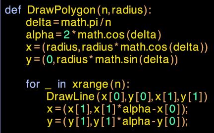
Appendix - Circle/Polygon drawing in Python

The following two functions are hereby licensed under CC0. 

# From http://missingbytes.blogspot.com/2012/05/circles.html
def DrawPolygon(n,centerX,centerY,radius):

    delta=math.pi/n

    twicecosdelta=2*math.cos(delta)

    x=(radius,radius*math.cos(delta))

    y=(0,radius*math.sin(delta))

    for _ in xrange(n):

        DrawLine(x[0]+centerX,y[0]+centerY,x[1]+centerX,y[1]+centerY)

        x=(x[1],x[1]*twicecosdelta-x[0]);

        y=(y[1],y[1]*twicecosdelta-y[0]);

# From http://missingbytes.blogspot.com/2012/05/circles.html
def DrawCircle(center,radius):

    maxError=0.5 # pixels

    n=int(math.ceil(2*math.pi/math.acos(1-maxError/radius)))

    DrawPolygon(n,center[0],center[1],radius)

Half-Open Squares

Allow me to re-introduce our friends, the half-open intervals :

The half-open interval,  [a,b)

They're the set of all x, such that a ≤ x and x < b.

We use them all the time.  Here's one :

An iterator in C++, over a half-open interval.

Open and Closed

What does it mean for a set to be open? What does it mean for it to be closed?  And half-open? What's up with that?

I'll save the formal definition for another time, but intuitively, we can think of an open set as one where every member has a little bit of wiggle room.  No matter how closely you zoom in to the edge of the set, there's always a little bit more before you get to the edge :

The open interval,  (a,b)

And a closed set? That's the set where if you start from the outside side of the set, there's always a little bit of wiggle room before you get to the edge. No matter how close to the edge of the set you are, there's always just a little bit of gap before you can get inside.

A set is closed iff its complement is open.

So half-open?  What's that?  Given the strange definitions for open and closed, it should come as no surprise we have another strange definition : A half-open set is one that has one side closed, and one side open!

Half open: one side closed, one side open.

Splitters and Joiners

Half open intervals are great for joining.  Suppose we have two half-open intervals, [a,b) and [b,c).  Then their union is just [a,c) .

Further more, if we know that if x is in [a,c), then it must be in either [a,b) or [b,c).

You'll see this all the time when we write recursive algorithms on containers with iterators, we use an iterator to split the container into two smaller containers, which each member is in one, and only one, of the children.

Rectangles

And what of the half-open rectangles?
Here's one:

1 ≤ x < 3 and  1 ≤ y < 3

If we use half-open rectangles, we get all of the same benefits as the 1 dimensional case.  We can easily form the union and intersection.  The empty rectangle has a simple representation.  We can subdivide, etc, etc

Here's what it might look like in code :

A Half-Open rectangle class.

Still not convinced?  Consider an 800 x 600 bitmap, whose pixels are [0,800) x [0,600)

for ( int y = 0; y < height; y++ )

{

    for ( int x = 0; x < width; x++ )

    {

        PlotPixel ( x, y, Color );

    }

}

Or this unbound function:

  Rectangle Intersect ( const Rectangle &a, const Rectangle &b )

  {
      return Rectangle (

          max ( a.X0, b.X0 ), max ( a.Y0, b.Y0 ),

          min ( a.X1, b.X1 ), min ( a.Y1, b.Y1 ) );
  }

Next time you make an interval, rectangle, or cube class, why not try using the half-open convention?  You'll almost certainly arrive at a smaller, more robust code.

Quadratic Formula

We all remember the quadratic formula from high school,  x = ( -b ± √ b² - 4ac ) / 2a, but if it's so familiar to us all of us, why do I keep coming across such bad implementations in code?

Polynomials

Lets start with a slightly more general problem, we're interested in finding all the real roots of these polynomials in x :

k₀  +  k₁ x  =  0

k₀  +  k₁ x  +  k₂ x²  =  0

k₀  +  k₁ x  +  k₂ x²  +  k₃ x³  =  0

k₀  +  k₁ x  +  k₂ x²  +  k₃ x³  +  k₄ x⁴   =  0

k₀  +  k₁ x  +  k₂ x²  +  k₃ x³  +  k₄ x⁴  +  k₅ x⁵  =  0

We know from the Fundamental Theorem Of Algebra that, for example, a quintic will have at most 5 real roots, so lets go ahead and write out the function prototypes :

(We also know from Galois Theory that quintics might require a numerical approximation, but that's a post for another day!)

The Quadratic Formula, Revisited

descriminant = kLinear² - 4*kQuadratic*kConstant

x = ( -kLinear ± √ descriminant ) / 2 / kQuadratic

So the first case that I hardly ever see handled, is when kQuadratic vanishes, leading to a divide-by-zero exception.  Actually, this case is very easy to handle if we have a family of functions:

Another important case is when kConstant is zero.  We can see graphically that the polynomial goes through the origin :

kConstant is zero means that 0.0 is a root.

Here's the code:

Note the sneaky 1+ and +1

Catastrophic Cancellation

The last problem we need to fix is when the square root of the descriminant is close in magnitude to kLinear.  Graphically :

This happens surprisingly often in physics calculations.

To fix this, consider the product of the roots :

rootProduct = root[0] * root[1]

rootProduct =  (-kLinear + √descriminant)/2/kQuadratic *

(-kLinear - √descriminant)/2/kQuadratic

rootProduct = ( -kLinear + √ descriminant ) * ( -kLinear - √ descriminant ) / 4 / kQuadratic²

Now something cool happens! Remember that (x+y) * (x-y) = x² - y²

rootProduct = ( (-kLinear)² - √ descriminant² ) / 4 / kQuadratic²

rootProduct = ( kLinear² - descriminant ) / 4 / kQuadratic²

Expanding:

rootProduct = ( kLinear² - kLinear² + 4*kQuadratic*kConstant) / 4 / kQuadratic²

rootProduct = ( kQuadratic*kConstant) / kQuadratic²

rootProduct = kConstant / kQuadratic

What this means is that we can use the larger root to calculate the smaller root by dividing by their product, and keep all the accuracy.

Appendix - Quadratic formula in C++

If you're just here for the code, the following two functions are hereby licensed under CC0. 

---

#include <math.h>
#define EPSILON (1e-10)

// From http://missingbytes.blogspot.com/2012/04/quadratic-formula.html
int SolveLinear(double rootDest[1],double kConstant,double kLinear){
    if(-EPSILON<kLinear&&kLinear<EPSILON){
        return 0;
    }
    rootDest[0]=-kConstant/kLinear;
    return 1;
}

// From http://missingbytes.blogspot.com/2012/04/quadratic-formula.html
int SolveQuadratic(double rootDest[2],double kConstant,double kLinear,double kQuadratic){
    if(-EPSILON<kQuadratic&&kQuadratic<EPSILON){
        return SolveLinear(rootDest,kConstant,kLinear);
    }
    if(-EPSILON<kConstant&&kConstant<EPSILON){
        rootDest[0]=0.0f;
        return 1+SolveLinear(rootDest+1,kLinear,kQuadratic);
    }
    double descriminant=kLinear*kLinear-4*kQuadratic*kConstant;
    if(descriminant<0){
        return 0;
    }
    if(descriminant==0){// no EPSILON check!!
        rootDest[0]=-kLinear/(2*kQuadratic);
        return 1;
    }
    double adder=sqrt(descriminant);
    if(adder*kLinear>0){
        adder=-adder;
    }
    double rootLarge=(-kLinear+adder)/(2*kQuadratic);
    rootDest[0]=rootLarge;
    rootDest[1]=kConstant/(kQuadratic*rootLarge);
    //std::sort(rootDest,rootDest+2);
    return 2;
}

---

Even More Math

They tell me that each mathematical formula in your blog post exactly halves your potential readership.

  How does that make you feel?

Why not talk about your feelings in the comments below?

Blur 90°

So I was refactoring recently, and came across this little gem.  We all know that separable filters can be computed in two passes, one pass in X, and a second pass in Y.  Naturally, that's actually what makes them separable.

The particular filter happened to be everybody's favorite, the 2 Dimensional Gaussian blur.

That's the filter that turns this :

Time and Date (in French), before..

Into this :

...and after, all blurred and ready for compositing.

Here's the Gaussian we're using, nothing fancy :

kernel(x,y) = exp( -x² + -y²)

And that same kernel in 1 dimension, looks like this :

1-dimensional Gaussian : exp(-x²)

This will be the filter we actually apply.

 

Straight Approach

Our straight forward approach would be to first filter in X, and then a second filter in Y.  Our sequence would look like this :

Well this is all well and good, but we'd end up writing two copies of the convolution code, each with different boundary conditions and memory access patterns.  That often leads to copy'n'paste-style duplicated code, and that can often lead to subtle bugs and swearing.

Sideways Approach

Here's the better way, as we filter, lets also rotate the bitmap 90°.

That is, we apply a filter that blurs in X, but also swaps the X and Y axis in the process.  Herein lies the magic, if we apply this filter twice, our original X-axis and Y-axis are restored, while our separable filter is applied to each axis in turn.

Here's the code if you're curious :

Yep, it really is that simple.

There's only one version of the convolution, so we can really put some good effort into checking our boundaries.

It's smaller code too, so less footprint in the instruction cache, and improved branch prediction, all good stuff for today's multi-threaded apps.

Shaders

If you're GPU bound, this works great for shaders too.  The performance of the actual filter will be the same, but you're running the same shader twice, so there's no expensive shader switching, especially if you're applying the same filter multiple times.

Of course, the big win here is removing duplication, so your shader will be more maintainable, easier to verify it's working correctly, and more robust if you use this technique.

Not just for Gaussian Blur

Of course, this technique works for any separable filter.  I also use rotate 90° in my high-quality bitmap scaling, and it works great - about 20% faster than the straight-forward approach, and much simpler code.

When profiling, one thing I found was slightly better cache performance by reading rows, and then writing columns. As always, profile on your own data to see what works best for you.

Results

Here's the final composite.  You can see the same effect applied to the pause ("paws") emblem in the top right. 

Bonus point if you can recognize the music video!

Comments

Now, I'm really sorry everyone, but the number of comments on this blog has been completely overwhelming and I simply can't keep up.  So even though the comments box below is working properly, I absolutely forbid you to post any comments, or discuss this post or blog in any way.

My apologies.