The Cacophony Index

Can we estimate the health of an ecosystem from a digital audio recording?

(Part 2 in a series about Artificial Intelligence and New Zealand native birds.)

Inside a computer, 20 seconds of audio are represented by a sequence of 320,000 numbers.

20 seconds of audio, plotted as a waveform

Our challenge is to take that series of 320,000 numbers and extract one single number, a "Cacophony Index", that has some special properties:

• Birds nearby and birds far away increase the Index about the same.
• Background noises don't affect the Index very much.
• The Cacophony Index for two sparrows chirping should be higher than if there's only one.
• The Cacophony Index for a sparrow chirping and an owl hooting should be higher than for two sparrows chirping.

Wow, that’s a really hard thing to do! As happens often in this blog, we'll make the problem easier by adding in some assumptions:

 "Perfect is the enemy of good" - Voltaire

Are we justified in making all these assumptions?
 ...Well, no...

...but...         

... let's do it anyway.

Lets build something useful instead of freaking out that a perfect solution can't exist.

That means we're going to just ignore a whole bunch of nasty complications like “clipping”, “nyquist rate”, “attenuation”, “noise floor”, etc

Because PROGRESS!

• Most of the loud noises in the recordings are birds, not people or cars or machines.
• The recording is “clean”
• The birds and the recorder stay in the same place.
• No running water or ocean waves (!)
• The recording was taken in New Zealand (!!)

Great stuff! Lets look at the spectrogram:

The spectrogram is a visual representation of the spectrum of frequencies of a signal as it varies with time. 

We don’t care so much about the intensity of any given bird call, that mostly tells us how near or far the bird is.

We don’t care so much if the bird has a short call or a long call.

Background noise? That’s where the spectrogram is well.. noisy..

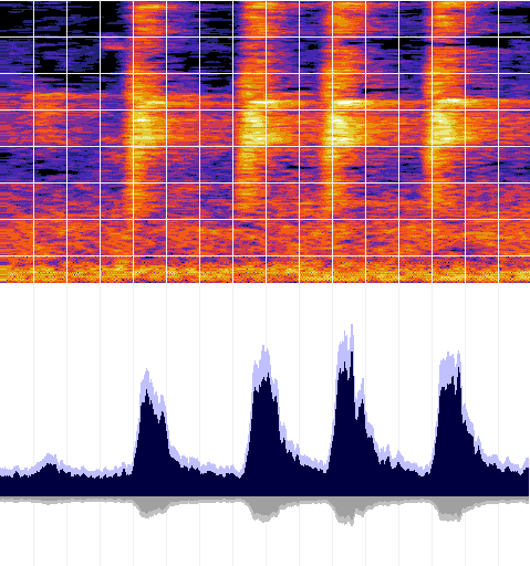
Count the number of times a yellow box is next to a blue box!
That's the heart of the Cacophony Index calculation.

What we’re really looking for is how the spectrogram changes over time.

Lets zoom in on that starting second and add a grid to isolate the signal in both time and frequency:

A little bit more math and we find the cacophony index for this particular audio recording is: 77

OK, you got me, I'm oversimplifying again!  ¯\_(ツ)\_/¯ If you want all the gory details, the code is on github.com

Lets talk Birds!

The Cacophony Index for 20 seconds of audio is just a number between zero and one hundred. By itself, not super useful.

If we make many recordings in the same location, we can plot how the Cacophony Index changes over time.  Here's one possible presentation of what that might look like over the course of a day:

You can clearly see the birds are more active during the day and less active during the night. The birds getting really noisy around sunrise and sunset, the "Dawn Chorus".

Even though the plot is a mock-up, the data is real. It's data from a real bird monitor, recorded near Christchurch, New Zealand over a three week period in November of 2019. We now have the technology to see how the Cacophony Index changes over a day, or a week, or even seasons, years or decades.

And that's exactly what the Cacophony Project are doing, using real audio recorded right here in New Zealand, uploaded continuously and automatically by people just like you! (Edit: Live! Check it out!)

I think that's awesome. Can we go deeper?

Now we have an automated way to track an ecosystem's health, what else can we do with the audio data?

Watch this space for an update using real AI using Tensorflow and some real world ethical problems.

Basic Income, Better Living Through Video Games.

If we assume as given we'll eventually live in a society with a UBI (all eligible citizens receive an Unconditional Basic Income, enough to cover their food, clothing and shelter), then the most pressing question is: How should we roll it out?

Years of making Video Games suggest two quick answers:

The easy way is by lottery. Suppose Gary is a winner in the monthly UBI Lottery! Congrats Gary! Gary no longer has to deal with our mess of confusing taxation and welfare regulations. He wins a much simplified UBI and a flat tax. Of course, any change can be scary and difficult, so Gary also has the option to just stick with the old system if he wants.

More interesting is the notion of a Dual Currency. It's a little bit like enrolling in the food stamp program, where he's issued with tokens that can be exchanged for food items at a 1-1 ratio. In a food stamp program, those tokens would normally expire after a set period of time.

Food stamps are really old. Like, 1930's America old. We live in a digital world, so lets make those tokens work more like an energy mechanic in Candy Crush or League of Legends. Those tokens now accrue *continuously* rather than appearing all at once on a Thursday. We'll cap Gary's balance at a maximum of 1 months worth of tokens. Any balance more than 2 weeks of tokens would also have a penalty applied.

Finally pricing. Staples like bread, milk, laundry detergent and cleaning supplies will have a heavily discounted price when purchased using tokens. Healthy options like fruit and vegetables too. Fast food and chocolates might have a premium pricing attached. Lets make it easier for Gary to make good decisions.

The Cap Theorem and Quantum Gravity

Apologies in advance, this post is both extremely technical in multiple fields, and woefully incomplete, and not nearly as humorous as it ought to be. Dragons be here. I'm incredibly sorry.

CAP Theorem for distributed systems

Brewer's CAP Theorem tells us that every distributed computer system must sacrifice at least one of these properties:

• C: Consistency
• A: Availability
• P: Partition Tolerance.

Astonishingly, if we view the universe as a distributed system, then Quantum Field Theory appears to have (analogues of) each of the three properties from the CAP theorem. But at what cost? Paradoxes. So many paradoxes. The double slit experiment, the twin paradox, the EPR “spooky action at a distance” paradox. Many many more. What if QFT adds to the CAP theorem a fourth property we could sacrifice:

• C: Consistency
• A: Availability
• P: Partition Tolerance
• T: Time Never Flows Backwards (!!!)

One Million Boulders

Lets look at that last one, Time Never Flows Backwards. Suppose, inside a computer, we're trying to simulate one million boulders rolling down a mountain side. At every time step, we need to generate all the potential collisions between those million boulders, and then process them in the order in which the collision occurs. You're familiar with Newton's cradle? Every one of those collisions can change the magnitude, and order, of any subsequent collision. And worse, round-off error when dicing the time steps means that a collision over *here* can affect a collision over *there*.

(All the gory details can be found here.)

Starting to sound a little bit like quantum dynamics right?

So how do we solve it efficiently? By briefly reversing the arrow of time. We find all the collisions between those boulders in a given timestep, then, optimistically, we solve each boulder independently (“in parallel”) based on it's known potential collisions, as if the order of collisions didn't matter. Then we do a “Fix-Up” phase where we wind the time step backwards and correct any of the boulders where (A) the collision order was incorrect, and (B) the energy of the correction is above a certain tolerance. (In practice the tolerance is very small, this tolerance only serves to prevent certain pathological worst-cases)

Starting to sound a *lot* like quantum dynamics...

Spinfoam

So imagine the spinfoam. In my mind, I visualize it something like this:

Spinfoam sketch, incomplete

In Quantum Chromo Dynamics terms, every face you can see is “Colourless” = (Red + Green + Blue == Red + Red + AntiRed + Green + Blue). In this diagram, the past is down. It's the rigid fixed lattice and appears unchangable. The future is a soup of these faces to the top of the diagram, and the “present” is the coalescing region where the mobile soup phase-transitions into a fixed lattice. Naturally, each edge is the Planck length, equivalently Plank time.

You can even see what we'd call a 'particle', maybe an electron or a neutrino, zipping along at close to the speed of light. In the spinfoam, it appears as a disturbance in the otherwise orderly lattice.

• <technical> In this diagram, the colours satisfy the Pauli exclusion principle. To represent bosons, simply write integer values at every vertex, and require every cycle-over-edges to sum to zero.
• This 2D diagram with vertices, edges and faces represents {1xspace+1xtime} dimensions. If we axiomatically accept the Holographic Principle, then it might be possible to represent {3xspace+1xtime} dimensions using only vertices, edges, faces and solids.</technical>

Notice too that, at least in the bottom of the diagram (“past”), the laws of physics are symmetric, and invariant under rotations through both time and space. Despite this local invariance, the time dimension can still be identified by it's global properties. The arrow of time, entropy etc, really does exist and has physical meaning.

Mass

What would happen if we tried to simulate this spinfoam in a computer? Well, most obvious to me, is that 'time' in the simulation does not correlate with the amount of computation required to run the simulation. Indeed, the computation required to run the simulation depends primarily on the search activity to coalesce the soup, and it should be easy to find a computation model where that search activity has a cost that matches Einstein's General Theory of Relativity. i.e. the curvature of a region of space is related to the amount of mass in that region, G = m . r^-2

Speed

Now lets take that simulation, and instead of running it on one single computer, we instead run it on a distributed computer system. Suddenly, the CAP theorem applies, and our simulation must sacrifice C, or A, or P.... or.... or..... or... T? What if we could sometimes run our simulation backwards just for a moment, the same as we did when "Fixing up" the simulate of those million boulders. When something doesn't fit, just for a little bit, we'd dissolve that fixed lattice of the past and turn it back into the mobile soup of the future, then reform the lattice into a consistent whole.
From inside the simulation, we'd never be able to send information back into the past (That would be a C violation!), and yet we'd still get “spooky action at a distance” and all those other paradoxes.
But at what cost? Well, surprisingly, only a performance hit. Again, it should be easy to find a model of distributed computation overhead where this performance hit is in exact agreement with Einstein's *Special* Theory of Relativity. Specifically, it's the Lorentz Transform, γ = 1 / sqrt(1-v².c^-2)

Intermission

Okay, big deep breath. The plot-twist is coming up soon. Brace yourself.

String Theory (Science Fiction)

Almost everything I've written above isn't new or novel. It's just a rehash of various discarded String-Theory ideas from the 90s, but with different names and labels. From an experimentalist physicists point of view, String Theory is just not that interesting. In terms of knowing more about the universe we live in, String Theory is pretty much at a dead end. Why? Because it's not *testable*. We can't devise an experiment in the lab to determine if any one of the thousands of competing String Theories makes predictions which match our unique reality. If your theory isn't testable, if there's no way to determine if you theory approximates our universe better than the alternatives, then that's not "Science" with a capital 'S', it's more like Science Fiction with a whole lot more math.

Plot Twist

So here's the plot-twist: CAP Theorem + QFT is testable.
Here's how: Take that exact same familiar double slit experiment we all faithfully reproduced when we first found out about Quantum Mechanics.

• Setup-1: Use one slit, fire the wave/particle, measure the diffraction. (Gaussian)
• Setup-2: Use two slits, fire the wave/particle, measure the diffraction. (Interference pattern)

Now, if we compare Setup-1 with Setup-2, if CAP + QFT is true, then Setup-2 will suffer a tiny time-dilation associated with resolving the CAP constraints. If CAP+QFT is true, we could toggle between Setup-1 and Setup-2 and measure the tiny difference in time dilation.

How tiny? So tiny no-one has ever noticed it before.

...so tiny, it would be much much smaller than the time-dilation associated with the mass of the photon itself.

......so tiny, but, at least in theory, so measurable.

What happens if we go into the lab and measure the time dilation difference between Setup-1 and Setup-2, and that difference turns out to be non-zero?

Quantum Gravity and Friends.

So yeah, that's a testable theory of quantum gravity. It neatly explains why gravity is so weak compared with the other forces (aka the Hierarchy problem), and dramatically simplifies the particle zoo.

Furthermore, this theorem is fully consistent with the Copenhagen Interpretation, and even builds on it! By contrast, In this formulation, the many-worlds alternative, however appears to have a vanishingly strict interpretation.

Black holes? Yip.. (I'll let you puzzle that one through, it's actually quite cute :) Naked singularities? Nope.

It neatly explains the uncertainty principle. It's truly a quantum theory from the get-go. The randomness is real ("no hidden variables"), it's even required, but it's certainly not arbitrary or capricious.

All those crazy dimensions from String Theory? Oh yeah, the dimensionality is there, but they're no longer spatial in nature, they're more like properties stacked on the spinfoam.

There's even some tantalising hints on the nature of dark matter and dark energy and inflation in the early universe..

Anyways, I've probably said way too much, as always, if you have any questions, queries or opinions, please let me know in the comments section below!

Twenty years of Skidmarks

Lately I've been digging through the old Skidmarks archives, and I came across this wee gem from 1993, no doubt written with lots of help from Simon:

Function.q hite {di.q,dj.q,oset.l}

  UNLK a4

  MOVE.l d2,a0

  MOVE.l d1,d2:SWAP d2:EXT.l d2:ASL.l #7,d2:ADD.l d2,a0

  MOVE.l d0,d2:SWAP d2:EXT.l d2:ASL.l #1,d2:ADD.l d2,a0

  MOVEM (a0)+,d2-d3 ;d0-d1 xy d2-d5 p0-p3

  LEA 124(a0),a0:MOVEM (a0)+,d4-d5

         MOVE d0,d6:MULU d1,d6:SWAP d6:MULU d6,d5  ; x. y.p3

  NOT d0:MOVE d0,d6:MULU d1,d6:SWAP d6:MULU d6,d4  ;-x. y.p2

  NOT d1:MOVE d0,d6:MULU d1,d6:SWAP d6:MULU d6,d2  ;-x.-y.p0

  NOT d0:           MULU d1,d0:SWAP d0:MULU d3,d0   ; x.-y.p1

  ADD.l d2,d0:ADD.l d4,d0:ADD.l d5,d0 ;total

  LSR.l#6,d0:RTS

End Function

For those not quite brave enough to decipher the 68000 assembly, here's what a strictly literal translation might be:

float Height(float x, float y, short *heightField){

  //__asm{...}

  heightField += int(x) * 64;

  heightField += int(y);

  short height2 = *heightfield++, height3 = *heightField++;

  heightField += 62; short height4=*heightfield++, height5 = *heightField++;

  float result5 = frac( x) * frac( y) * height5;

  float result4 = frac(-x) * frac( y) * height4;

  float result2 = frac(-x) * frac(-y) * height2;

  float result0 = frac( x) * frac(-y) * height0;

  float result = (result0 + result2 + result4 + result5);
  return result / 64;

}

The motivation is that I've been working towards a new version for mobile devices, with a working title of "Super Skidmarks 2000" (hashtag #SS2K)

Here's what the modern version of that same function looks like, this time in C++ :

float SKTrack::GetHeight(float axisI,float axisJ)const{

  int fi=(int)floor(axisI);

  int fj=(int)floor(axisJ);

  if(fi<0||fi>=63){

    return 0.0f;

  }

  if(fj<0||fj>=63){

   return 0.0f;

  }

  int index=fi+fj*64;

  float v0=HeightField[index];

  float v1=HeightField[index+1];

  float v2=HeightField[index+64];

  float v3=HeightField[index+65];

  float s=axisI-floor(axisI);

  float t=axisJ-floor(axisJ);

  float v01=v0*(1.0f-s)+v1*s;

  float v23=v2*(1.0f-s)+v3*s;

  float height=v01*(1.0f-t)+v23*t;

  return height;

}

As always, any questions / comments, or suggestion for a better name etc, please leave a comment below!

The Infinite Blogpost

There's an Indie project floating around at the moment, that's being touted as infinite.

For some reason, it really bugs me when people take a perfectly good word, a word like "infinite", and then apply it incorrectly.

You see, a desktop computer is finite.

Suppose your desktop computer is a Commodore VIC-20, with a whopping 3.5 kilobytes of memory.  Then there are only 256^3,583 different states that your desktop computer can be in.

Sure, that's a lot of states, but it's certainly not infinite. You could, at least in principle, enumerate them all.  And you'd find that there are exactly 256^3,583 of them.  That's the very definition of finite.

Finite software runs on finite computers

Lets take a closer look at those finite states on the VIC-20.  We know that the computer is finite, but maybe there is some magical technique in which we could write a computer program to have an infinite amount of state?

Unfortunately, no, we cannot.  The pigeon hole principle forbids it.

Fast forward to the Modern Era

Oh? Your computer has more memory than a VIC-20? 4 Gigabytes perhaps?

Well that's still just 256^{4,294,967,296} states.  It's still not infinite.

Oh, you have a 3TB hard drive as well?

Okay, so now you have access to an additional 256^{3,298,534,883,328} different states.

That's a lot of storage.  These numbers are large, but they're all still finite.

The problem is that infinity is just so mindbogglingly larger than any number you could possibly store on your hard drive.

You'd need a technology shift to be able to store infinite state.

Bandwidth, over time, is Infinite

So hopefully I've managed to convince you that your computer, and by extension, the software running on it, is finite. Regardless of what that hardware is.

But now consider, the curious case of your internet connection.

If you're like me, you have a bandwidth cap of 4GB per month.  Then it is true, that for any particular month, your bandwidth is finite.

But consider your 4GB bandwidth extending over time.

I can send 8GB in 2 months.  Or 40GB in 10 months. Or 400GB in 100 months.

Here's the curious thing, if we assume that time is infinite (a big assumption, granted), then for any amount of state, we can calculate how many months it would take to send that state on your internet connection by dividing by 256^{4,294,967,296} .


Let me repeat that, given any amount of state, we could send that state in a finite amount of time, over your internet connection.

And that is what is meant by "Bandwidth, over time, is infinite".

The Cocktail Party Effect (Part 2 of 2)

Late at night, when the boys are (finally) asleep, we like to be able to hear the voices of the people on the television without waking up the neighbors.  In part one I described how to build a custom digital audio filter by specifying a frequency response and running an optimizer to determine the optimal coefficients.

This post looks at one of the actual filters I use on my television in more detail.

First up, here's the response curve for the filter.

White = Filter,   Blue=Desired Response

You can see the extremely strong cut-off starting at 1000Hz, dropping very quickly, -10 dB at 300Hz, and -20dB at 50Hz.  In the other direction, we have an almost flat response between 1000Hz and 5000Hz, and then a very gradual drop, -3dB at 10kHz.

This corresponds nicely with the human voice, which ranges between 800Hz - 8000Hz, with the majority of the sound energy between 1500Hz-4000Hz

Here's the actual code I use to set the desired frequency:

    float GetDesiredResponse(float freq)

    {
        float logFreq = log(freq);
        float cutOff0 = log(1000.0f);
        float cutOff1 = log(3400.0f);
        float cutOff2 = log(8000.0f);

        float result = 1.0f;
        if(logFreq  < cutOff0)

        {
            float factor = logFreq / cutOff0;
            result *= pow(factor, 10.0f);
        }
        if(logFreq > cutOff1)

        {
            float factor = 2.0f - logFreq / cutOff1;
            result *= pow(factor, 2.0f);
        }
        if(logFreq > cutOff2)

        {
            float factor = 2.0f - logFreq / cutOff2;
            result *= pow(factor, 2.0f);
        }
        return result;
    }

As you can see with this method, it's relatively easy to get precise control over the frequency response.

A couple quick notes:

• It's important that the frequency response be a quasiconcave function.  This ensures there are no kinks in the response, which will (1) cause visiting audiophiles to complain, and (2) make some voices more difficult to comprehend.

• Be careful when specifying a very steep transition, or trying to completely stop-pass some frequencies.  A digital filter has some pretty strict limits on the kinds of things it can filter.  Like the proverbial genie, if you try and go there, the optimizer will give you exactly what you ask for.
  

• I can't hear past ~17kHz, so I took extra care to test with high frequencies, but played back at half speed to make sure I wasn't torturing the cats and dogs.
  

• This is also a good time to read up about Odd and Even functions, which correspond to odd/even numbers of coefficients in the polynomial.  An Odd function, for example, will start at -∞ and rise to +∞.  That's useful if you want a high-pass or low-pass filter, but bad for a band-pass filter.

• Having problems with the y racing off to infinity? Your Y polynomial may have an unstable feedback loop.  Try a longer or shorter filter, or add an A-stability criteria to your optimizer.

 

Weighting

So you're probably wondering why the filter matches the desired function so accurately over the vocal range, but seems to drift in other areas.  Here's the weighting function I use to compute the error:

That is, I sample 129 frequencies logarithmically spaced between 9Hz to 18000Hz.  For each frequency, I add the square of the L2 error, weighted by the square of (desired response + a quarter).

Why so much squaring?  To help the function minimizer converge to a global minimum, it's nice to give big parabolas for the optimizer to slide inside.

Oh, and before I forget, here's the actual filter in C++, licensed under CC0:

    // From http://missingbytes.blogspot.com/2012/06/cocktail-party-effect-part-2-of-2.html
    static float x[5] = {0};
    for(int i=0; i<length; i++)
    {
        float sampleLeft = GetNextLeftSample();
        float sampleRight = GetNextRightSample();

        for(int j=4; j>0; j--)
        {
            x[j] = x[j-1];
        }
        x[0] = sampleLeft + sampleRight;

        // The filter!
        static float y1=0.0f, y2=0.0f, y3=0.0f, y4=0.0f;
        f32 y0=+0.588746*x[0]-0.492725*x[1]-0.757061*x[2]+0.661062*x[3]
            +1.242758*y1+0.545942*y2-1.044236*y3+0.238844*y4;
        y4=y3;y3=y2;y2=y1;y1=y0;

        float value = y0*volume;
        float outValue = bound(value, -32768, 32767);
        if(value != outValue){clippingCount++;}
        unsigned short emit = (unsigned short)outValue;
        *dest++ = emit;// Output left
        *dest++ = emit;// Output right
    }

Results

So what does it sound like?  Well, for music, pretty bad actually :)  But that's not the point!  It's designed for voice, and that where it really shines - even though the voice quality sounds a little unnatural, you can understand what people are saying, even at very low volume levels.

    (Oops, having some video encoding problems - updated video coming real soon now)

The Future

Can we do better than this?  Yes, we can!  When I finally get around to setting up a 7.1 audio system, I plan to measure the room response function using a calibrated microphone.  Then it's a simple matter of taking the FFT of the incoming audio, dividing through by the room response, then taking the inverse fourier transform before sending to the sound card.  Normally this would entail some delay/lag, but that's not a problem when playing buffered video.  I could even have different responses for different listener locations, or dynamically respond to changes in temperature or humidity.

... watch this space for a future update.

The Cocktail Party Effect (Part 1 of 2)

Late at night, when the boys are (finally) asleep, we sometimes like to watch stuff on the television.  If the TV is too loud, the boys wake up, and that really breaks immersion.  If the TV is too quiet, we can't hear the gripping dialogue, and that breaks immersion too.

  Here's how I fixed it in code.

Mono

Okay. Don't judge me, but the first thing I did is to convert the incoming stereo audio down to mono.  Most music tends to be well spatialised, while the voice track comes through the center channel.  By converting to mono I estimate a ~3dB drop in perceived volume during musical interludes, or, conversely, I can raise the total volume by 3dB without waking up the boys.

Bass

The next thing to do is to cut the low frequencies.  The rumbles and the explosions.  The ones which reverberate throughout the house and wake up the kids and the neighbors too.

It's relatively easy to find info on constructing a digital high-pass filter on the internet, provided you can cut through the jargon.  Generally there tends to be an incoming signal, denoted as x_n.  It's the series of samples coming from your video decoder.  And then there's an outgoing signal, y_n.  It's the series of samples that you send to the sound card.

Then there's some function that links them together.  Here's an example of a really simple high-pass filter you can find on the internet :

y_n = 0.2 . x_n  + 0.8 . y_n-1

It's a simple matter to turn this into code:

A simple high-pass filter, in C++.

Z-transform

To work out the frequency response, we can use the Z-transform to find the Transfer Function, which maps our filter from the discrete, time domain, into the continuous, frequency domain.  In our case:

H(z) = Y(z)/X(z) =  0.2 / (1 + 0.8 . z^-1)

The cool thing is we can use theory to treat z like a complex number, even though in practice, all the x_n and y_n will be floating point numbers.  For example, to compute the frequency response at 1000Hz, with a sample rate of 48kHz, we take:

i = √-1

FrequencyResponse(1000Hz) = | H(2π1000/48000 i) |

= | 0.2/(1 + 0.8 / (2π1000i/48000) ) |

= 0.008

If we draw this on a graph, with frequency (Hz) on the X-axis, and magnitude (dB) on the Y-axis, we can get a "Bode Plot" of our filter:

A Bode Plot for a simple filter.

So that's a great start, but now we want more control over which frequencies pass through the filter, and which are blocked, and by how much.

Optimize

Back in the old days, we would have had to endlessly try different filter combinations and painstakingly compute Bode plots to find combinations of filters that might fit our requirements.

But now that we all have super-computers under our desks, we've got much more powerful tools to solve an old problem in a new way.

In pseudo-code, it looks like this :

def GetDesiredFrequencyResponse(frequency):

    // Your desired EQ function goes here

def EvaluateFilter(filter):

    errorSum = 0

    for frequency in 20 .. 22000:

        freq1 = GetDesiredFrequencyResponse(frequency)

        freq2 = filter.CalcFrequencyResponse(frequency)

        errorTerm = freq1 - freq2

        errorSum += errorTerm * errorTerm

    return errorSum

bestFilter = Minimize(FilterFactory, EvaluateFilter)

That's right, lets just use an offline optimizer to compute the optimal co-efficients for us!  You could use numpy, or octave for this.

... And Generate the Code

'f32' is a 32-bit float

Now we have our filter coefficients, we need to inject it back into C++.

Here's a function which writes out the C++ directly.  We can just copy and paste directly into  ProcessAudio(), hit recompile, and hear the results immediately.

Notice the coding style - it's rife with buffer overflows, and makes huge unjustified assumptions about the inputs.  You certainly couldn't use this code in a production environment, but as the scaffolding to bootstrap a single-use filter, the iteration speed trumps all other considerations.

Sample

Here's a sample output :

    static float y1 = 0.0f, y2 = 0.0f;
    float sum = 0.211989*x[0]
        -6.794531*x[-1]
        -29.803024*x[-2]
        +0.535980*x[-3]
        +0.215555*x[-4];
    float y0 = (sum -9.433180*y1 +31.500277*y2) / 0.000017;
    y2 = y1;
    y1 = y0;

Coming Soon

So this is part 1 of 2, in the next post I'll go into the details of the actual filters I'm using on my television, as well as some sample video so you can hear before and after.  I'll try and include tips for how to ensure convergence, and some gotchas that the Bode plot won't tell you about.  And of course, if there's anything you'd like to know more, why not suggest it in the comments below?

Circles

I was recently reading @dubejf's post on generating a sin lookup table, and it reminded me of a really old technique for circle drawing, inspired by the CORDIC algorithm.

A circle rasterized on a bitmap.

Circle

In the Platonic sense, a circle is the set of all points a given distance from the origin.

As always, the Platonic ideal is unobtainable.

But for those of us fortunate enough to be stuck on the inside of a computer, we're happy to settle for an approximation instead.

Normally when I'm in a raster environment, I use the excellent Bresenham circle algorithm.  It's integer-only, and runs great on embedded devices where memory access is slow, but random access is okay.

On the other hand, if I need an anti-aliased circle and have enough silicon available, I tend to use a signed distance representation.  It's much better suited for pixel shaders and is great for feature discovery when compositing.

But this post is about a different method altogether, it approximates a circle by a polygon, and then draws that polygon instead.  It works best in vector environments, or for drawing arcs, or custom line effects, or, well, any time it's easier to draw polygons than to push pixels. Like over a remote desktop connection for example.

Anyway, lets see the algorithm, and then you can decide where it best fits in your toolbox!

Computing the maximum error.

Error term

One technique I use all the time, is to limit the error to be less than half a pixel. This way my approximation is visually indistinguishable from the ideal circle. It also makes for a great free parameter if you later need to optimize at the expense of a little quality.

Lets go ahead and calculate the error term now.

For a polygon with N vertices, let δ be the angle between each vertex:

δ = 2 π / N

Then the maximum deviation between the circle and the approximating polygon is given by:

error_max = radius . (1 - cos(δ/2) )

 Now we can go ahead and bound it from above by 0.5 pixels:

radius . (1 - cos(δ/2) ) ≤ error  ≤ 0.5 (pixels)

We can combine these equations to figure out the number of vertices our polygon needs.

N  ≥  π / cos ^-1(1 - 0.5 / radius)  

So now we can draw an N-sided polygon to approximate our circle, with error less than half a pixel, and it should be visually indistinguishable from the platonic ideal :

Draw a circle by using an approximating polygon.

Just to get a feel for how many vertices we're talking about, here's radius (pixels) and N (vertices) for a few select values:

radius	N
6	8
9	10
13	12
20	15
30	18
45	22
68	26

Polygon Drawing (The Easy Way)

Well we all know one easy way to draw a polygon, lets just generate the co-ordinates for each vertex in turn, and then draw lines between them.  Something like this :

def DrawEasyPolygon(n, radius):
    prevPosition = (radius, 0)
    for i in xrange(n):
        angle = (i+1) * 2 * math.pi
        x = math.cos(angle) * radius
        y = math.sin(angle) * radius
        position = (x,y)

        DrawLine(prevPosition, position)

        prevPosition = position

But can we do better than that?  If only there was some way to get rid of all those calls to math.sin and math.cos inside the loop.

A recurrence formula for the sin function

 

Lets start with the angle sum and difference formulas:

• sin( θ + δ ) = cos δ sin θ  + sin δ cosθ
• sin( θ - δ ) = cos δ sin θ  - sin δ cosθ

We can add these together and rearrange to reveal:

• sin( θ + δ )  = 2 cos δ sin θ  - sin( θ - δ )

Or, rewriting as a recurrence relation :

α = 2 cos δ
x_n+1 =  α x_n - x_n-1

Here's what that looks like in code:

Generate a sin table, using a recurrence relation.

So now we have a little bit of trigonometry to setup, but then our entire inner loop consists of a multiply, a subtract and some register shuffling.

Incidentally this particular recurrence formula has excellent error properties. It seems you can run this recurrence forever without losing magnitude, and only a tiny predictable phase shift.  (Part of it comes from this being a so-called "symplectic" method, but it seems to perform even better than that.  I have a suspicion this particular recurrence somehow squeezes out the error during it's zero-crossing.  If I have time in the future I'd love to investigate further.)

Polygon Drawing (The Good Way)

So now we can combine our recurrence relation with our previous polygon draw:

The good way of drawing a polygon.

Some whimsical polygonal circles.

Results

Well, as you can see, we have circles!  Just for fun, I alternated drawing blue and red lines to highlight the individual line segments a little more clearly.

There's probably a little more we could do here, it looks like the maxError should maybe be lowered a little, and we may want to force N to be a multiple of four to enforce symmetry.

We'd also want to trap for very small and very large circles, and maybe tweak the polygon radius to better match the circle's radius.

Also, keep in mind our error condition, if you zoom in to this image, the error will be much bigger than a pixel and much more noticeable.

This caveat is equally applicable if you're using super-sampling.  Be sure to modify your error constraints appropriately.

But I'll leave all these extra concerns for the comments section down below.

---

Appendix - Circle/Polygon drawing in Python

The following two functions are hereby licensed under CC0. 

# From http://missingbytes.blogspot.com/2012/05/circles.html
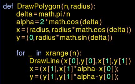
def DrawPolygon(n,centerX,centerY,radius):

    delta=math.pi/n

    twicecosdelta=2*math.cos(delta)

    x=(radius,radius*math.cos(delta))

    y=(0,radius*math.sin(delta))

    for _ in xrange(n):

        DrawLine(x[0]+centerX,y[0]+centerY,x[1]+centerX,y[1]+centerY)

        x=(x[1],x[1]*twicecosdelta-x[0]);

        y=(y[1],y[1]*twicecosdelta-y[0]);

# From http://missingbytes.blogspot.com/2012/05/circles.html
def DrawCircle(center,radius):

    maxError=0.5 # pixels

    n=int(math.ceil(2*math.pi/math.acos(1-maxError/radius)))

    DrawPolygon(n,center[0],center[1],radius)

Half-Open Squares

Allow me to re-introduce our friends, the half-open intervals :

The half-open interval,  [a,b)

They're the set of all x, such that a ≤ x and x < b.

We use them all the time.  Here's one :

An iterator in C++, over a half-open interval.

Open and Closed

What does it mean for a set to be open? What does it mean for it to be closed?  And half-open? What's up with that?

I'll save the formal definition for another time, but intuitively, we can think of an open set as one where every member has a little bit of wiggle room.  No matter how closely you zoom in to the edge of the set, there's always a little bit more before you get to the edge :

The open interval,  (a,b)

And a closed set? That's the set where if you start from the outside side of the set, there's always a little bit of wiggle room before you get to the edge. No matter how close to the edge of the set you are, there's always just a little bit of gap before you can get inside.

A set is closed iff its complement is open.

So half-open?  What's that?  Given the strange definitions for open and closed, it should come as no surprise we have another strange definition : A half-open set is one that has one side closed, and one side open!

Half open: one side closed, one side open.

Splitters and Joiners

Half open intervals are great for joining.  Suppose we have two half-open intervals, [a,b) and [b,c).  Then their union is just [a,c) .

Further more, if we know that if x is in [a,c), then it must be in either [a,b) or [b,c).

You'll see this all the time when we write recursive algorithms on containers with iterators, we use an iterator to split the container into two smaller containers, which each member is in one, and only one, of the children.

Rectangles

And what of the half-open rectangles?
Here's one:

1 ≤ x < 3 and  1 ≤ y < 3

If we use half-open rectangles, we get all of the same benefits as the 1 dimensional case.  We can easily form the union and intersection.  The empty rectangle has a simple representation.  We can subdivide, etc, etc

Here's what it might look like in code :

A Half-Open rectangle class.

Still not convinced?  Consider an 800 x 600 bitmap, whose pixels are [0,800) x [0,600)

for ( int y = 0; y < height; y++ )

{

    for ( int x = 0; x < width; x++ )

    {

        PlotPixel ( x, y, Color );

    }

}

Or this unbound function:

  Rectangle Intersect ( const Rectangle &a, const Rectangle &b )

  {
      return Rectangle (

          max ( a.X0, b.X0 ), max ( a.Y0, b.Y0 ),

          min ( a.X1, b.X1 ), min ( a.Y1, b.Y1 ) );
  }

Next time you make an interval, rectangle, or cube class, why not try using the half-open convention?  You'll almost certainly arrive at a smaller, more robust code.

Quadratic Formula

We all remember the quadratic formula from high school,  x = ( -b ± √ b² - 4ac ) / 2a, but if it's so familiar to us all of us, why do I keep coming across such bad implementations in code?

Polynomials

Lets start with a slightly more general problem, we're interested in finding all the real roots of these polynomials in x :

k₀  +  k₁ x  =  0

k₀  +  k₁ x  +  k₂ x²  =  0

k₀  +  k₁ x  +  k₂ x²  +  k₃ x³  =  0

k₀  +  k₁ x  +  k₂ x²  +  k₃ x³  +  k₄ x⁴   =  0

k₀  +  k₁ x  +  k₂ x²  +  k₃ x³  +  k₄ x⁴  +  k₅ x⁵  =  0

We know from the Fundamental Theorem Of Algebra that, for example, a quintic will have at most 5 real roots, so lets go ahead and write out the function prototypes :

(We also know from Galois Theory that quintics might require a numerical approximation, but that's a post for another day!)

The Quadratic Formula, Revisited

descriminant = kLinear² - 4*kQuadratic*kConstant

x = ( -kLinear ± √ descriminant ) / 2 / kQuadratic

So the first case that I hardly ever see handled, is when kQuadratic vanishes, leading to a divide-by-zero exception.  Actually, this case is very easy to handle if we have a family of functions:

Another important case is when kConstant is zero.  We can see graphically that the polynomial goes through the origin :

kConstant is zero means that 0.0 is a root.

Here's the code:

Note the sneaky 1+ and +1

Catastrophic Cancellation

The last problem we need to fix is when the square root of the descriminant is close in magnitude to kLinear.  Graphically :

This happens surprisingly often in physics calculations.

To fix this, consider the product of the roots :

rootProduct = root[0] * root[1]

rootProduct =  (-kLinear + √descriminant)/2/kQuadratic *

(-kLinear - √descriminant)/2/kQuadratic

rootProduct = ( -kLinear + √ descriminant ) * ( -kLinear - √ descriminant ) / 4 / kQuadratic²

Now something cool happens! Remember that (x+y) * (x-y) = x² - y²

rootProduct = ( (-kLinear)² - √ descriminant² ) / 4 / kQuadratic²

rootProduct = ( kLinear² - descriminant ) / 4 / kQuadratic²

Expanding:

rootProduct = ( kLinear² - kLinear² + 4*kQuadratic*kConstant) / 4 / kQuadratic²

rootProduct = ( kQuadratic*kConstant) / kQuadratic²

rootProduct = kConstant / kQuadratic

What this means is that we can use the larger root to calculate the smaller root by dividing by their product, and keep all the accuracy.

Appendix - Quadratic formula in C++

If you're just here for the code, the following two functions are hereby licensed under CC0. 

---

#include <math.h>
#define EPSILON (1e-10)

// From http://missingbytes.blogspot.com/2012/04/quadratic-formula.html
int SolveLinear(double rootDest[1],double kConstant,double kLinear){
    if(-EPSILON<kLinear&&kLinear<EPSILON){
        return 0;
    }
    rootDest[0]=-kConstant/kLinear;
    return 1;
}

// From http://missingbytes.blogspot.com/2012/04/quadratic-formula.html
int SolveQuadratic(double rootDest[2],double kConstant,double kLinear,double kQuadratic){
    if(-EPSILON<kQuadratic&&kQuadratic<EPSILON){
        return SolveLinear(rootDest,kConstant,kLinear);
    }
    if(-EPSILON<kConstant&&kConstant<EPSILON){
        rootDest[0]=0.0f;
        return 1+SolveLinear(rootDest+1,kLinear,kQuadratic);
    }
    double descriminant=kLinear*kLinear-4*kQuadratic*kConstant;
    if(descriminant<0){
        return 0;
    }
    if(descriminant==0){// no EPSILON check!!
        rootDest[0]=-kLinear/(2*kQuadratic);
        return 1;
    }
    double adder=sqrt(descriminant);
    if(adder*kLinear>0){
        adder=-adder;
    }
    double rootLarge=(-kLinear+adder)/(2*kQuadratic);
    rootDest[0]=rootLarge;
    rootDest[1]=kConstant/(kQuadratic*rootLarge);
    //std::sort(rootDest,rootDest+2);
    return 2;
}

---

Even More Math

They tell me that each mathematical formula in your blog post exactly halves your potential readership.

  How does that make you feel?

Why not talk about your feelings in the comments below?