The Cacophony Index

Can we estimate the health of an ecosystem from a digital audio recording?

(Part 2 in a series about Artificial Intelligence and New Zealand native birds.)

Inside a computer, 20 seconds of audio are represented by a sequence of 320,000 numbers.

20 seconds of audio, plotted as a waveform

Our challenge is to take that series of 320,000 numbers and extract one single number, a "Cacophony Index", that has some special properties:

• Birds nearby and birds far away increase the Index about the same.
• Background noises don't affect the Index very much.
• The Cacophony Index for two sparrows chirping should be higher than if there's only one.
• The Cacophony Index for a sparrow chirping and an owl hooting should be higher than for two sparrows chirping.

Wow, that’s a really hard thing to do! As happens often in this blog, we'll make the problem easier by adding in some assumptions:

 "Perfect is the enemy of good" - Voltaire

Are we justified in making all these assumptions?
 ...Well, no...

...but...         

... let's do it anyway.

Lets build something useful instead of freaking out that a perfect solution can't exist.

That means we're going to just ignore a whole bunch of nasty complications like “clipping”, “nyquist rate”, “attenuation”, “noise floor”, etc

Because PROGRESS!

• Most of the loud noises in the recordings are birds, not people or cars or machines.
• The recording is “clean”
• The birds and the recorder stay in the same place.
• No running water or ocean waves (!)
• The recording was taken in New Zealand (!!)

Great stuff! Lets look at the spectrogram:

The spectrogram is a visual representation of the spectrum of frequencies of a signal as it varies with time. 

We don’t care so much about the intensity of any given bird call, that mostly tells us how near or far the bird is.

We don’t care so much if the bird has a short call or a long call.

Background noise? That’s where the spectrogram is well.. noisy..

Count the number of times a yellow box is next to a blue box!
That's the heart of the Cacophony Index calculation.

What we’re really looking for is how the spectrogram changes over time.

Lets zoom in on that starting second and add a grid to isolate the signal in both time and frequency:

A little bit more math and we find the cacophony index for this particular audio recording is: 77

OK, you got me, I'm oversimplifying again!  ¯\_(ツ)\_/¯ If you want all the gory details, the code is on github.com

Lets talk Birds!

The Cacophony Index for 20 seconds of audio is just a number between zero and one hundred. By itself, not super useful.

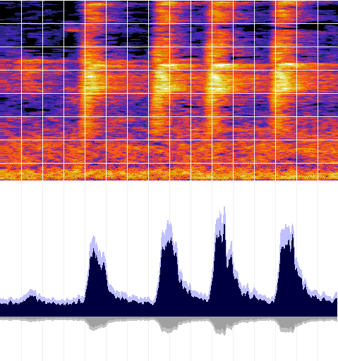
If we make many recordings in the same location, we can plot how the Cacophony Index changes over time.  Here's one possible presentation of what that might look like over the course of a day:

You can clearly see the birds are more active during the day and less active during the night. The birds getting really noisy around sunrise and sunset, the "Dawn Chorus".

Even though the plot is a mock-up, the data is real. It's data from a real bird monitor, recorded near Christchurch, New Zealand over a three week period in November of 2019. We now have the technology to see how the Cacophony Index changes over a day, or a week, or even seasons, years or decades.

And that's exactly what the Cacophony Project are doing, using real audio recorded right here in New Zealand, uploaded continuously and automatically by people just like you! (Edit: Live! Check it out!)

I think that's awesome. Can we go deeper?

Now we have an automated way to track an ecosystem's health, what else can we do with the audio data?

Watch this space for an update using real AI using Tensorflow and some real world ethical problems.

ShiftP

Buddy of mine wants to straighten some images automatically, kinda like ShiftN :



Oh, you'll want Python version 2, I said:

#makefile
PIP2=pip
PYTHON2=python

setup2:
$(PIP2) install --user virtualenv
$(PYTHON2) -m virtualenv v2
source v2/bin/activate && pip install numpy Pillow pylsd

And Python 3, I said, also in a VirtualENVironment sandbox:

#makefile
PIP3=pip3
PYTHON3=python3

setup3:
#$(PYTHON3) -m venv v3
source v3/bin/activate && pip install numpy Pillow scipy

setup: setup2 setup3
-mkdir temp

run:
source v2/bin/activate && python FindLines.py Source.jpg

source v3/bin/activate && python Warp.py

Start by finding all your lines:

#FindLines.py
import json
import numpy
import sys

from PIL import Image
import pylsd.lsd

def ExportMeta(fileName,outName):
meta={'fileName':fileName}
image=Image.open(fileName)
meta['width']=image.width
meta['height']=image.height
grayScale=numpy.asarray(image.convert('L'))
lines=pylsd.lsd(grayScale)
lineArray=[]
for row in lines:
lineArray.append(list(row))
meta['lineArray']=lineArray

with open(outName,'w') as f:
f.write(json.dumps(meta,sort_keys=True,separators=(',', ': '),indent=4))


ExportMeta(sys.argv[1],'temp/meta.json')

Always prefilter your inputs, I nagged:

#Warp.py
def FindWeightedLines(lineArray,meta):
linesHorizontal=[]
linesVertical=[]
for (x0,y0,x1,y1,width) in lineArray:
if width<2:
continue
h0=RemapXY(x0,y0,meta)
h1=RemapXY(x1,y1,meta)
dx=abs(h0[0]-h1[0])
dy=abs(h0[1]-h1[1])
if max(dx,dy)<min(dx,dy)*4:
continue
magnitude=dx*dx+dy*dy
if dx<dy:
linesHorizontal.append([magnitude,h0,h1])
else:
linesVertical.append([magnitude,h0,h1])

return sorted(linesHorizontal)[-30:]+sorted(linesVertical)[-30:]
#Always prefilter your inputs!!!

Now here's the tricksy bit, in *TWO* parts, setup a perspective transform:

#Warp.py
def RemapXY(x,y,meta):
xx=(x-meta['width']/2)/meta['scale']
yy=(y-meta['height']/2)/meta['scale']
return (xx,yy,1)

def UnmapXYZ(xx,yy,zz,meta):
rx=xx/zz
ry=yy/zz
x=rx*meta['scale']+meta['width']/2
y=ry*meta['scale']+meta['height']/2
return (x,y)

*And* a non-linear warp. We don't need the full power of Chebyshev Polynomials here, I reminded him. We can just use 0, 1, x, y, x², y² and xy. Why? Because all spanning basis-es are equivalent in low dimensions!

#Warp.py
def ApplyTransform(transform,x,y,z):
rx=x*transform[0]+y*transform[1]+z*transform[2]
ry=x*transform[3]+y*transform[4]+z*transform[5]
rz=x*transform[6]+y*transform[7]+z*transform[8]
nonLinear=True
if nonLinear:
rx+=x*y*transform[9]
ry+=x*y*transform[10]
rx+=x*x*transform[11]
ry+=x*x*transform[12]
rx+=y*y*transform[13]
ry+=y*y*transform[14]
return (rx,ry,rz)

def ApplyTransformhomogenous(transform,x,y,z):
(hx,hy,hz)=ApplyTransform(transform,x,y,z)
return (hx/hz,hy/hz)

Next you'll need a loss function, weakly constrain your transform matrix, then setup a sum-of-squares for your error term:

#Warp.py
def loss(transform,meta):

result=0

for i in range(9):

t=transform[i]

if i==0 or i == 4 or i == 8:

t=transform[i]-1

result += t*t

for(weight,h0,h1) in meta['weightedLineArray']:

(x2,y2)=ApplyTransformHomogenous(transform,*h0)

(x3,y3)=ApplyTransformHomogenous(transform,*h1)

dx=abs(x3-x2)

dy=abs(y3-y2)

if dx<dy:
(dx,dy)=(dy,dx)
q=math.sqrt(dx*dx + dy*dy)
dx=dx/q
dy=dy/q

result += dy*dy

Are we done yet? Oh, a driver...:

#Warp.py
def Main():
with open('temp/meta.json','r') as f:
meta=json.loads(f.read())
meta['scale']=math.sqrt(meta['width']*meta['height'])/2

meta['weightedLineArray']=FindWeightedLines(meta['lineArray'],meta)

m=minimize(loss,[1,0,0,0,1,0,0,0,1,0,0,0,0,0,0],args=meta)

transform=m.x

(x0,y0,x1,y1) = FindClipRectangle(...)

source=Image.open(meta['fileName'])

image=Image.new('RGB',(x1-x0,y1-y0),(0,0,0))

draw=ImageDraw.Draw(image)

meta['splitCount']=64

for x in range(meta['splitCount']):

for y in range(meta['splitCount']):

p00=SquareMap(x,y,meta)

p01=SquareMap(x,y+1,meta)

p10=SquareMap(x+1,y,meta)

p11=SquareMap(x+1,y+1,meta)

r00=ApplyTransform(transform,*RemapXY(*p00,meta))

r01=ApplyTransform(transform,*RemapXY(*p01,meta))

r10=ApplyTransform(transform,*RemapXY(*p10,meta))

r11=ApplyTransform(transform,*RemapXY(*p11,meta))

s00=UnmapXYZ(*r00,meta)

s01=UnmapXYZ(*r01,meta)

s10=UnmapXYZ(*r10,meta)

s11=UnmapXYZ(*r11,meta)

TextureMapTriangle(draw,x0,y0,x1,y1,source,s00,s01,s10,p00,p01,p10)

TextureMapTriangle(draw,x0,y0,x1,y1,source,s10,s01,s11,p10,p01,p11)

print('Progress %d/%d'%(x,meta['splitCount']),flush=True)

image.save('temp/warped.jpg')

Oh, and you need texture mapped triangles? Python is terrible for that, there's no way to make it run fast.... Fine, here's one of those, just to get you started, but don't blame me if it's slow, this needs to be in OpenGL or something so you can run it on the GPU and apply proper gamma correction.

#TextureMapTriangle.py
def Left(p,a,b):
cross=(p[0]-a[0])*(b[1]-a[1])-(p[1]-a[1])*(b[0]-a[0])
return cross<0

def SampleMap(source,x,y,dx,dy):
if x<0:
x=0
if y<0:
y=0
if x>=source.width:
x=source.width-1
if y>=source.height:
y=source.height-1
return source.getpixel((x,y))


def TextureMapTriangle(draw,x0,y0,x1,y1,source,p0,p1,p2,uv0,uv1,uv2):
xy0=list(map(min,zip(p0,p1,p2)))
xy1=list(map(max,zip(p0,p1,p2)))

dx1=p1[0]-p0[0]
dy1=p1[1]-p0[1]
dx2=p2[0]-p0[0]
dy2=p2[1]-p0[1]
det=dx1*dy2-dx2*dy1
if xy0[0]<x0:
xy0[0]=x0
if xy0[1]<y0:
xy0[1]=y0
if xy1[0]>x1:
xy1[0]=x1
if xy1[1]>y1:
xy1[1]=y1

for x in range(math.floor(xy0[0]),math.ceil(xy1[0])):
for y in range(math.floor(xy0[1]),math.ceil(xy1[1])):
p=(x,y)
if Left(p,p0,p1):
continue
if Left(p,p1,p2):
continue
if Left(p,p2,p0):
continue

dx=x-p0[0]
dy=y-p0[1]
u=(dx*dy2-dy*dx2)/det
v=(-dx*dy1+dy*dx1)/det

uu=uv0[0]+u*(uv1[0]-uv0[0])+v*(uv2[0]-uv0[0])
vv=uv0[1]+u*(uv1[1]-uv0[1])+v*(uv2[1]-uv0[1])
c=SampleMap(source,uu,vv,1,1)
draw.point((x-x0,y-y0),tuple(c))

And then you could be like me, and license all of the above code under CC0. Yay!

Twenty years of Skidmarks

Lately I've been digging through the old Skidmarks archives, and I came across this wee gem from 1993, no doubt written with lots of help from Simon:

Function.q hite {di.q,dj.q,oset.l}

  UNLK a4

  MOVE.l d2,a0

  MOVE.l d1,d2:SWAP d2:EXT.l d2:ASL.l #7,d2:ADD.l d2,a0

  MOVE.l d0,d2:SWAP d2:EXT.l d2:ASL.l #1,d2:ADD.l d2,a0

  MOVEM (a0)+,d2-d3 ;d0-d1 xy d2-d5 p0-p3

  LEA 124(a0),a0:MOVEM (a0)+,d4-d5

         MOVE d0,d6:MULU d1,d6:SWAP d6:MULU d6,d5  ; x. y.p3

  NOT d0:MOVE d0,d6:MULU d1,d6:SWAP d6:MULU d6,d4  ;-x. y.p2

  NOT d1:MOVE d0,d6:MULU d1,d6:SWAP d6:MULU d6,d2  ;-x.-y.p0

  NOT d0:           MULU d1,d0:SWAP d0:MULU d3,d0   ; x.-y.p1

  ADD.l d2,d0:ADD.l d4,d0:ADD.l d5,d0 ;total

  LSR.l#6,d0:RTS

End Function

For those not quite brave enough to decipher the 68000 assembly, here's what a strictly literal translation might be:

float Height(float x, float y, short *heightField){

  //__asm{...}

  heightField += int(x) * 64;

  heightField += int(y);

  short height2 = *heightfield++, height3 = *heightField++;

  heightField += 62; short height4=*heightfield++, height5 = *heightField++;

  float result5 = frac( x) * frac( y) * height5;

  float result4 = frac(-x) * frac( y) * height4;

  float result2 = frac(-x) * frac(-y) * height2;

  float result0 = frac( x) * frac(-y) * height0;

  float result = (result0 + result2 + result4 + result5);
  return result / 64;

}

The motivation is that I've been working towards a new version for mobile devices, with a working title of "Super Skidmarks 2000" (hashtag #SS2K)

Here's what the modern version of that same function looks like, this time in C++ :

float SKTrack::GetHeight(float axisI,float axisJ)const{

  int fi=(int)floor(axisI);

  int fj=(int)floor(axisJ);

  if(fi<0||fi>=63){

    return 0.0f;

  }

  if(fj<0||fj>=63){

   return 0.0f;

  }

  int index=fi+fj*64;

  float v0=HeightField[index];

  float v1=HeightField[index+1];

  float v2=HeightField[index+64];

  float v3=HeightField[index+65];

  float s=axisI-floor(axisI);

  float t=axisJ-floor(axisJ);

  float v01=v0*(1.0f-s)+v1*s;

  float v23=v2*(1.0f-s)+v3*s;

  float height=v01*(1.0f-t)+v23*t;

  return height;

}

As always, any questions / comments, or suggestion for a better name etc, please leave a comment below!

The Cocktail Party Effect (Part 2 of 2)

Late at night, when the boys are (finally) asleep, we like to be able to hear the voices of the people on the television without waking up the neighbors.  In part one I described how to build a custom digital audio filter by specifying a frequency response and running an optimizer to determine the optimal coefficients.

This post looks at one of the actual filters I use on my television in more detail.

First up, here's the response curve for the filter.

White = Filter,   Blue=Desired Response

You can see the extremely strong cut-off starting at 1000Hz, dropping very quickly, -10 dB at 300Hz, and -20dB at 50Hz.  In the other direction, we have an almost flat response between 1000Hz and 5000Hz, and then a very gradual drop, -3dB at 10kHz.

This corresponds nicely with the human voice, which ranges between 800Hz - 8000Hz, with the majority of the sound energy between 1500Hz-4000Hz

Here's the actual code I use to set the desired frequency:

    float GetDesiredResponse(float freq)

    {
        float logFreq = log(freq);
        float cutOff0 = log(1000.0f);
        float cutOff1 = log(3400.0f);
        float cutOff2 = log(8000.0f);

        float result = 1.0f;
        if(logFreq  < cutOff0)

        {
            float factor = logFreq / cutOff0;
            result *= pow(factor, 10.0f);
        }
        if(logFreq > cutOff1)

        {
            float factor = 2.0f - logFreq / cutOff1;
            result *= pow(factor, 2.0f);
        }
        if(logFreq > cutOff2)

        {
            float factor = 2.0f - logFreq / cutOff2;
            result *= pow(factor, 2.0f);
        }
        return result;
    }

As you can see with this method, it's relatively easy to get precise control over the frequency response.

A couple quick notes:

• It's important that the frequency response be a quasiconcave function.  This ensures there are no kinks in the response, which will (1) cause visiting audiophiles to complain, and (2) make some voices more difficult to comprehend.

• Be careful when specifying a very steep transition, or trying to completely stop-pass some frequencies.  A digital filter has some pretty strict limits on the kinds of things it can filter.  Like the proverbial genie, if you try and go there, the optimizer will give you exactly what you ask for.
  

• I can't hear past ~17kHz, so I took extra care to test with high frequencies, but played back at half speed to make sure I wasn't torturing the cats and dogs.
  

• This is also a good time to read up about Odd and Even functions, which correspond to odd/even numbers of coefficients in the polynomial.  An Odd function, for example, will start at -∞ and rise to +∞.  That's useful if you want a high-pass or low-pass filter, but bad for a band-pass filter.

• Having problems with the y racing off to infinity? Your Y polynomial may have an unstable feedback loop.  Try a longer or shorter filter, or add an A-stability criteria to your optimizer.

 

Weighting

So you're probably wondering why the filter matches the desired function so accurately over the vocal range, but seems to drift in other areas.  Here's the weighting function I use to compute the error:

That is, I sample 129 frequencies logarithmically spaced between 9Hz to 18000Hz.  For each frequency, I add the square of the L2 error, weighted by the square of (desired response + a quarter).

Why so much squaring?  To help the function minimizer converge to a global minimum, it's nice to give big parabolas for the optimizer to slide inside.

Oh, and before I forget, here's the actual filter in C++, licensed under CC0:

    // From http://missingbytes.blogspot.com/2012/06/cocktail-party-effect-part-2-of-2.html
    static float x[5] = {0};
    for(int i=0; i<length; i++)
    {
        float sampleLeft = GetNextLeftSample();
        float sampleRight = GetNextRightSample();

        for(int j=4; j>0; j--)
        {
            x[j] = x[j-1];
        }
        x[0] = sampleLeft + sampleRight;

        // The filter!
        static float y1=0.0f, y2=0.0f, y3=0.0f, y4=0.0f;
        f32 y0=+0.588746*x[0]-0.492725*x[1]-0.757061*x[2]+0.661062*x[3]
            +1.242758*y1+0.545942*y2-1.044236*y3+0.238844*y4;
        y4=y3;y3=y2;y2=y1;y1=y0;

        float value = y0*volume;
        float outValue = bound(value, -32768, 32767);
        if(value != outValue){clippingCount++;}
        unsigned short emit = (unsigned short)outValue;
        *dest++ = emit;// Output left
        *dest++ = emit;// Output right
    }

Results

So what does it sound like?  Well, for music, pretty bad actually :)  But that's not the point!  It's designed for voice, and that where it really shines - even though the voice quality sounds a little unnatural, you can understand what people are saying, even at very low volume levels.

    (Oops, having some video encoding problems - updated video coming real soon now)

The Future

Can we do better than this?  Yes, we can!  When I finally get around to setting up a 7.1 audio system, I plan to measure the room response function using a calibrated microphone.  Then it's a simple matter of taking the FFT of the incoming audio, dividing through by the room response, then taking the inverse fourier transform before sending to the sound card.  Normally this would entail some delay/lag, but that's not a problem when playing buffered video.  I could even have different responses for different listener locations, or dynamically respond to changes in temperature or humidity.

... watch this space for a future update.

The Cocktail Party Effect (Part 1 of 2)

Late at night, when the boys are (finally) asleep, we sometimes like to watch stuff on the television.  If the TV is too loud, the boys wake up, and that really breaks immersion.  If the TV is too quiet, we can't hear the gripping dialogue, and that breaks immersion too.

  Here's how I fixed it in code.

Mono

Okay. Don't judge me, but the first thing I did is to convert the incoming stereo audio down to mono.  Most music tends to be well spatialised, while the voice track comes through the center channel.  By converting to mono I estimate a ~3dB drop in perceived volume during musical interludes, or, conversely, I can raise the total volume by 3dB without waking up the boys.

Bass

The next thing to do is to cut the low frequencies.  The rumbles and the explosions.  The ones which reverberate throughout the house and wake up the kids and the neighbors too.

It's relatively easy to find info on constructing a digital high-pass filter on the internet, provided you can cut through the jargon.  Generally there tends to be an incoming signal, denoted as x_n.  It's the series of samples coming from your video decoder.  And then there's an outgoing signal, y_n.  It's the series of samples that you send to the sound card.

Then there's some function that links them together.  Here's an example of a really simple high-pass filter you can find on the internet :

y_n = 0.2 . x_n  + 0.8 . y_n-1

It's a simple matter to turn this into code:

A simple high-pass filter, in C++.

Z-transform

To work out the frequency response, we can use the Z-transform to find the Transfer Function, which maps our filter from the discrete, time domain, into the continuous, frequency domain.  In our case:

H(z) = Y(z)/X(z) =  0.2 / (1 + 0.8 . z^-1)

The cool thing is we can use theory to treat z like a complex number, even though in practice, all the x_n and y_n will be floating point numbers.  For example, to compute the frequency response at 1000Hz, with a sample rate of 48kHz, we take:

i = √-1

FrequencyResponse(1000Hz) = | H(2π1000/48000 i) |

= | 0.2/(1 + 0.8 / (2π1000i/48000) ) |

= 0.008

If we draw this on a graph, with frequency (Hz) on the X-axis, and magnitude (dB) on the Y-axis, we can get a "Bode Plot" of our filter:

A Bode Plot for a simple filter.

So that's a great start, but now we want more control over which frequencies pass through the filter, and which are blocked, and by how much.

Optimize

Back in the old days, we would have had to endlessly try different filter combinations and painstakingly compute Bode plots to find combinations of filters that might fit our requirements.

But now that we all have super-computers under our desks, we've got much more powerful tools to solve an old problem in a new way.

In pseudo-code, it looks like this :

def GetDesiredFrequencyResponse(frequency):

    // Your desired EQ function goes here

def EvaluateFilter(filter):

    errorSum = 0

    for frequency in 20 .. 22000:

        freq1 = GetDesiredFrequencyResponse(frequency)

        freq2 = filter.CalcFrequencyResponse(frequency)

        errorTerm = freq1 - freq2

        errorSum += errorTerm * errorTerm

    return errorSum

bestFilter = Minimize(FilterFactory, EvaluateFilter)

That's right, lets just use an offline optimizer to compute the optimal co-efficients for us!  You could use numpy, or octave for this.

... And Generate the Code

'f32' is a 32-bit float

Now we have our filter coefficients, we need to inject it back into C++.

Here's a function which writes out the C++ directly.  We can just copy and paste directly into  ProcessAudio(), hit recompile, and hear the results immediately.

Notice the coding style - it's rife with buffer overflows, and makes huge unjustified assumptions about the inputs.  You certainly couldn't use this code in a production environment, but as the scaffolding to bootstrap a single-use filter, the iteration speed trumps all other considerations.

Sample

Here's a sample output :

    static float y1 = 0.0f, y2 = 0.0f;
    float sum = 0.211989*x[0]
        -6.794531*x[-1]
        -29.803024*x[-2]
        +0.535980*x[-3]
        +0.215555*x[-4];
    float y0 = (sum -9.433180*y1 +31.500277*y2) / 0.000017;
    y2 = y1;
    y1 = y0;

Coming Soon

So this is part 1 of 2, in the next post I'll go into the details of the actual filters I'm using on my television, as well as some sample video so you can hear before and after.  I'll try and include tips for how to ensure convergence, and some gotchas that the Bode plot won't tell you about.  And of course, if there's anything you'd like to know more, why not suggest it in the comments below?

Circles

Recently I was reading @missingbytes' post about drawing a circle by approximating it with a polygon, and it got me to thinking, how would you draw a circle on the GPU?

Circle

In the previous post, a circle is drawn using an explicit formula :

(x, y)  =  radius . (cos θ, sin θ)

θ ∊ [0, 2π)

In this post, we're going to start with the implicit form :

x² + y² - radius² = 0

Which we then convert into a signed distance :

s(x, y) = x² + y² - radius²

Which can then be normalized by dividing through by the derivative at the zero crossing:

s(x, y) = ( x² + y² - radius² ) / 2.radius

We can visualize that signed distance function by mapping the signed distance directly to intensity :

Signed distance function for a circle

From here we can convolve with a sinc function and immediately get our circle :

sinc(x) = sin(x) / x

In code, that looks like this :

But can we do better than that?  If you recall the Nyquist-Shannon sampling theorem, we can only recover a signal whose frequency is less than half the sample rate.  At the moment, we're pushing frequencies at exactly that limit.  Some people like the look of that "poppiness" or "crunchiness", but personally, I prefer to back away a little bit from the limit and try to leave at least 20% head room :

float alpha = sinc ( s * Pi * 0.8 );

And what of those negative lobes and moire patterns?  Lets chop them off:

float WindowedSinc(float x)
{

    if (x <= -3.1415926 ) { return 0; }

    if (x >= 3.1415926 ) { return 0; }

    if (x == 0 ) { return 1; }

    return sin(x) / x;

}

One last consideration, we need to consider the transfer function and gamma of the monitor.  Luckily, we can approximate this by taking the square root!

return float4( 1, 1, 1, sqrt(alpha) );

Results

 On the right is our finished circle, aliased to 80% of the nyquist limit and with approximate gamma correction.  For comparison, I've also included the circles from the earlier post on the left.

Modern GPU Programming

I've used HLSL and DirectX in this post, but this technique works equally well in OpenGL.  With only slight modifications, you can even use this technique on OpenGL ES on the iPad or Android.

Hopefully this post has given you a bit of a flavor for some of the considerations in modern GPU programming. If you'd like to know more, or have any suggestions for improvements, please let me know in the comments below!

---

Appendix - Circle drawing in HLSL

The following three functions are hereby licensed under CC0. 

float radius;
float2 center;
float3 strokeColor;

# From http://missingbytes.blogspot.com/2012/05/circles_12.html

float WindowedSinc(float x){

    if(x<=-Pi){return 0;}

    if(x>=Pi){return 0;}

    if(x==0){return 1;}

    return sin(x)/x;

}

# From http://missingbytes.blogspot.com/2012/05/circles_12.html
float GammaCorrectAlpha(float3 color,float alpha){

    float a=1-sqrt(1-alpha);

    float b=sqrt(alpha);

    float t=(color.x+color.y+color.z)/3;

    return a*(1-t)+b*t;

}

# From http://missingbytes.blogspot.com/2012/05/circles_12.html
float4 CirclePixelShader(in float2 screenPosition:TEXCOORD):COLOR{
    float xx=uv.x-screenPosition.x;
    float yy=uv.y-screenPosition.y;
    float s=(xx*xx+yy*yy-radius*radius)/2/radius;
    float alpha=WindowedSinc(s*Pi*0.8);
    float alphaScreen=GammaCorrectAlpha(strokeColor,alpha);
    return float4(strokeColor.xyz,alphaScreen);
}

Blur 90°

So I was refactoring recently, and came across this little gem.  We all know that separable filters can be computed in two passes, one pass in X, and a second pass in Y.  Naturally, that's actually what makes them separable.

The particular filter happened to be everybody's favorite, the 2 Dimensional Gaussian blur.

That's the filter that turns this :

Time and Date (in French), before..

Into this :

...and after, all blurred and ready for compositing.

Here's the Gaussian we're using, nothing fancy :

kernel(x,y) = exp( -x² + -y²)

And that same kernel in 1 dimension, looks like this :

1-dimensional Gaussian : exp(-x²)

This will be the filter we actually apply.

 

Straight Approach

Our straight forward approach would be to first filter in X, and then a second filter in Y.  Our sequence would look like this :

Well this is all well and good, but we'd end up writing two copies of the convolution code, each with different boundary conditions and memory access patterns.  That often leads to copy'n'paste-style duplicated code, and that can often lead to subtle bugs and swearing.

Sideways Approach

Here's the better way, as we filter, lets also rotate the bitmap 90°.

That is, we apply a filter that blurs in X, but also swaps the X and Y axis in the process.  Herein lies the magic, if we apply this filter twice, our original X-axis and Y-axis are restored, while our separable filter is applied to each axis in turn.

Here's the code if you're curious :

Yep, it really is that simple.

There's only one version of the convolution, so we can really put some good effort into checking our boundaries.

It's smaller code too, so less footprint in the instruction cache, and improved branch prediction, all good stuff for today's multi-threaded apps.

Shaders

If you're GPU bound, this works great for shaders too.  The performance of the actual filter will be the same, but you're running the same shader twice, so there's no expensive shader switching, especially if you're applying the same filter multiple times.

Of course, the big win here is removing duplication, so your shader will be more maintainable, easier to verify it's working correctly, and more robust if you use this technique.

Not just for Gaussian Blur

Of course, this technique works for any separable filter.  I also use rotate 90° in my high-quality bitmap scaling, and it works great - about 20% faster than the straight-forward approach, and much simpler code.

When profiling, one thing I found was slightly better cache performance by reading rows, and then writing columns. As always, profile on your own data to see what works best for you.

Results

Here's the final composite.  You can see the same effect applied to the pause ("paws") emblem in the top right. 

Bonus point if you can recognize the music video!

Comments

Now, I'm really sorry everyone, but the number of comments on this blog has been completely overwhelming and I simply can't keep up.  So even though the comments box below is working properly, I absolutely forbid you to post any comments, or discuss this post or blog in any way.

My apologies.